Model Predictive Control

What is it?

Basic overview

Model Predictive Control (MPC) is a method of control that essentially simulates a short time into the future, and chooses the inputs that produce the best future. This relies on two things: the dynamics of the system, and the optimization constraints.

The dyamics of the system are what allow it to simulate possible futures. The more accurate the dynamics, the more accurate the simulated future will be. However, the more complex the dynamics are, the more computationally expensive it will be to run the simulations and optimization. Our system is heavily nonlinear, which means it will be very complex.

The optimization constraints determine which future will be chosen. The constraints inform the system about which inputs are possible, and which outputs are ideal. For example, the constraints might say that keeping the car close to the path is good, going fast is good, and hitting cones is bad. Then, the most optimal future will be one that stays close to the path while driving fast and not hitting any cones.

We will be using the dynamics and optimization constraints described in this paper.

Videos

The first five videos in this series by MATLAB explains MPC conceptually: MPC videos by MATLAB

This video goes more in-depth about MPC: MPC video by Steve Brunton

Dynamics

The dynamics of the car are modeled as a dynamic bicycle model with nonlinear tire force laws. The model holds under four assumptions: the vehicle drives on a flat surface, load transfer can be neglected, combined slip can be neglected, and the longitudinal drive-train forces can be neglected.

The final system dyanmics consists of the linear combination of two different models, a dynamical model and a kinematic model. This is because the dynamical model is not accurate at low speeds due to slip angles. Similarly, the kinematic model is not accurate at high speeds because they neglect the interaction between the tires and ground. A linear combination of the two models allows both models to be used in their ideal regions.

Dynamical model

The dynamical model is accurate at high speeds:

$alt dyn eqn$

The states and parameters are defined in the "Variables and parameters" section below.

Kinematic model

The kinematic model is accurate at low speeds. Note how it uses both $utilde$ and $utildedot$ as inputs:

$alt kin eqn$

The states and parameters are defined in the "Variables and parameters" section below.

Blended model

The final model is given by a linear combination of the dynamical model and kinematic model. At high speeds, the entire dynamical model will be used. At low speeds, the entire kinematic model will be used. In between, a mix of the dynamical and kinematic model will be used:

$alt final eqn$

$lambda$ is a blending parameter defined in the "Variables and parameters" section below.

Variables and parameters

For reference, here is an image of the bicycle model with all parameters. You don't need to understand everything about it, but it can be useful to look at.

Bicycle model

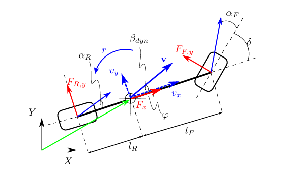
The state of the model is $xtilde = [X, Y, phi, vx, vy, r]^T$ . The individual states are defined as:

$(X, Y)$ , the 2D coordinates of the center of the car
$phi$ , the heading of the car
$vx$ , the x (longitudal) velocity of the center of the car
$vy$ , the y (lateral) velocity of the center of the car
$r$ , the yaw rate (angular velocity) of the car

The control input is $utilde = [delta, D]^T$ . The individual inputs are defined as:

$delta$ , the steering angle
$D in [-1, 1]$ , the driving command. 1 for full throttle, -1 for full braking

Note that the kinematic model depends on $utildedot$ . We discretize $utildedot = del utilde$ , where $del utilde = [del D, del delta]^T$ . In the optimization problem, it is assumed that we can only control $del utilde$ .

The parameters used in the dynamical and kinematic models are as follows:

$m$ , the mass of the car
$m$ , the intertia
$l_r$ , the distance from the center of gravity to the rear wheel
$l_f$ , the distance from the center of gravity to the front wheel
$F_R,y$ , the lateral tire force of the rear wheel
- - $alpha_R eqn$ , the rear slip angle
  - $B_R, C_R, D_R$ are experimentally identified coefficients
$F_F,y$ , the lateral tire force of the front wheel
- $F_F,y eqn$
  - $alpha_F eqn$ , the front slip angle
  - $B_F, C_F, D_F$ are experimentally identified coefficients
$F_x$ , the longitudinal combined force produced by the drivetrain
- $F_x = C_m D - C_r0 - C_r2 v_x^2$
  - $C_m D$ , the experimentally identified motor model
  - $C_r9$ , the experimentally identified rolling resistance
  - $C_r2$ , the experimentally identified drag coeficcient
$tau_TV$ , the additional moment produced by the torque vectoring system
- $tau_TV = (r_target - r)P_TV$
  - $r_target = delta(v_x / l_F + l_R$ , the kinematic yaw rate
  - $P_TV$ , the proportional gain of the low level torque vectoring controller
$lambda$ , the blending parameter
- $alt blend eqn$
  - $v_x,blend min$ , the velocity below which the kinematic modely is purely used. Determined to be 3 m/s
  - $v_x,blend max$ , the velocity above which the dynamical modely is purely used. Determined to be 5 m/s

Optimization

The final optimization problem will be structured as a constrained optimization problem. This means that there will be an objective function that will be minimized, subject to contstraints.

The objective function will be constructed from several cost functions, which each govern a part of how we choose the optimal solution. As evidenced by the name, the higher the cost function is, the worse our car is performing, which is why we try to minimize the cost.

The constraints will mostly be physical constraints that our car is subject to, such as the maximum force the tires can exert and the limits of the track (cones).

Contouring formulation

The goal of the contouring formulation is to follow the path given to us as closely as possible. It is assumed that the path is given by a function that allows us to compute a point on the path $(X_ref(theta),Y_ref(theta))$ with a variable. To follow the path, the position of the car must be linked to a point on the path, which is the arc-length $theta_p$ . However, it is computationally too expensive to find the true arc-length $theta_p$ , so instead we introduce a new state $theta$ which approximates the arc length. This approximation is given by a double integrator:

$\color{white}\theta=\int_{0}^{t}\dot{\theta}dt=\int_{0}^{t}v_{\theta}dt=\int_{0}^{t}\int_{0}^{t}\dot{v_{\theta}}dtdt$

$thetadot = v_theta$ , the velocity of the car relative to the reference path
$v_theta dot = del v_theta$ , the acceleration of the car relative to the reference path

Note that $theta$ is the double integral of acceleration, which results in a position.

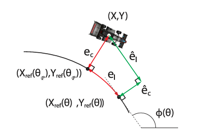
To keep $theta$ as a good approximation of the true $theta_p$ , we construct a cost function which minimizes the error, given by:

$J cost eqn$

With parameters:

$e_c$ , the contouring error, the error perpendicular to the reference path
- $e_c eqn$
  - $Phi(theta)$ , the angle of the tangent to the reference path at point $theta$
$e_l$ , the lag error, the error along to the reference path
- $e_c eqn$
  - $Phi(theta)$ , the angle of the tangent to the reference path at point $theta$
$q_c, q_l, gamma$ , weights $>= 0$ on the objectives

Note that this cost function minimizes the errors $e_l$ and $e_c$ while maximizing the velocity along the path $v_theta$ .

This image shows how the error looks on the path.

Contour Formulation errors

Cost functions

We can construct further cost functions that help to choose the optimal future. The first is a penalty to control inputs:

$control penalty eqn$

The second is a slip slide angle cost, which controls the aggressiveness of the MPC:

$slip slide angle cost eqn$

The parameters for these two cost functions are:

$R_u$ , a matrix which defines the cost of each control input
$R_del u$ , a matrix which defines the cost of changing each control input
$beta_kin$ , the kinematic slide slip angle
- $beta_kin = arctan(tan(delta)l_R / l_R + l_F)$
$beta_dyn$ , the dynamic slide slip angle
- $beta_dyn = arctan(v_y/v_x)$

Tire constraints

To simplify the dynamical bicycle model, it was assumed that combined slip can be neglected. However, this is not strictly true. A tire has a maximum elliptice force budget it can transfer to the ground, called the friction ellipse. This budget can be introduced as a constraint, which allows us to ignore combined slip in our dynamical model. The constraints are given by:

$tire eqn 1$

$tire eqn 2$

with parameters

$p_long$ , tire specific ellipse parameter. Lowering this parameter allows the vehicle to corner more while accelerating
$p_ellipse$ , tire specific ellipse parameter. Increasing this parameter allows the vehicle to go closer to the force limit

Track constraints

We must add constraints to the MPC problem that tell it to stay within the track boundaries. The constraint is given by:

$track eqn$

with parameters:

$R_Track(theta)$ , the safe radius around the track at point $theta$ .
$S_c$ , a slack variable to soften the constraint, which may be needed to guarantee the equation is solvable

With the addition of a slack variable $S_c$ , we can define a final cost function:

$C(S_c) = q_s S_c + q_ss S_c^2$

with parameters:

$q_s, q_ss$ , weights $>= 0$ that penalize the use of the slack variable

Final MPC Problem

Finally, we can construct our MPC problem. We can combine vehicle model, input dynamics, and arc-length dynamics into one equation:

$xfinal eqn$

We then discretize the system as:

$\color{white}{\mathbf{x}}_{k+1}=f(\mathbf{x}_{k},\Delta\mathbf{u}_k)$

Which allows us to write our final MPC problem, with a prediction horizon of N:

$final problem!!$

Our MPC problem can now be solved using an optimization solver. The output is $delta u$ , which we can apply to our control inputs.

Model Predictive Control

What is it?

Basic overview

Videos

Dynamics

Dynamical model

Kinematic model

Blended model

Variables and parameters

Optimization

Contouring formulation

Cost functions

Tire constraints

Track constraints

Final MPC Problem

Optimization package

TBD

What is it?​

Basic overview​

Videos​

Dynamics​

Dynamical model​

Kinematic model​

Blended model​

Variables and parameters​

Optimization​

Contouring formulation​

Cost functions​

Tire constraints​

Track constraints​

Final MPC Problem​

Optimization package​

TBD​

What is it?

Basic overview

Videos

Dynamics

Dynamical model

Kinematic model

Blended model

Variables and parameters

Optimization

Contouring formulation

Cost functions

Tire constraints

Track constraints

Final MPC Problem

Optimization package

TBD